You use this program to view the Available to Promise (ATP) details for a specific stock code/warehouse combination.
The sales department can use this program to check that they do not sell what the purchasing and production departments cannot supply. The production planning department can use the program (as an alternative to the pegging details) to establish the effects of a change in supply on demand emanating from higher levels of the product being constructed.
The ATP enquiry allows the viewing of the uncommitted portion of the stock. It is calculated up to and including the date of the planning time fence.
This program can be run at any time.
If you are new to this query, then the following information will help you achieve the best results:
-
If you know the stock code, then you can enter it directly and press the Tab or Enter key to view the information.
If you do not know the stock code, then you can use the browse function to locate the code.
-
You can personalize this query in a number of ways. These include:
- configuring property sheets (e.g. the section headed Stock Code Information). This includes being able to sequence items by dragging them up or down, to show important items first
- configuring the Details listview. This includes being able to sequence columns by dragging them left or right, sorting columns and changing column widths
- configuring the layout of the panes on the screen, including hiding or displaying panes
- Toolbar and menu
- List of warehouses
- ATP
- Sample calculations
- Stock Code Information
- Details
- Notes and warnings
| Field | Description |
|---|---|
| Options | |
| MPS | This generates the supply of an MPS item from the build schedule. |
| Non MPS | This generates the supply of an MPS item from jobs and purchase orders. |
| Stock code | Enter the stock code for which you want to display the
information. You cannot view details for a stock item defined as a Notional part (Stock Codes). |
| Find | Select this to use the Key Search program to locate items according to extensive search criteria. |
| Change date | Select this to enter a different run date for the ATP
calculation. Enter the date in CCYY/MM/DD format. This field is disabled when an invalid stock code is entered in the Stock code field. |
| Change Rev/Rel | Select this to change the revison/release for an ECC
controlled stock item. This field is disabled if an invalid stock code is entered in the Stock code field or when a non ECC controlled stock code is used. |
As you highlight a warehouse, the information in the ATP pane and the Details listview is refreshed to display the information for that warehouse.
![[Note]](images/note.png)
|
|
|
Only warehouses to which you are allowed access are displayed (Operators). |
|
This displays the ATP information for the warehouse currently highlighted in the List of Warehouses pane.
MPS items (Stock Codes) include the build schedules as supply.
For non-MPS items, purchase orders are included when the purchase order status is 0, 1 or 4, the purchase order is active and incomplete, and there is a quantity outstanding. The purchase order date is calculated as Purchase order due date + dock to stock for the item (non-working days are taken into account for the dock to stock).
The ATP for each period is calculated as follows:
-
In the first period:
The starting on hand balance + net requirements build schedule quantity (SUPPLY) - [sales orders + job allocations (DEMAND) for the same period, plus periods prior to the next net requirements build schedule.]
-
For subsequent periods:
Net requirements build schedules for the period - sales orders and job allocations for the same period plus periods prior to the next net requirements build schedule.
| Column | Description | ||||
|---|---|---|---|---|---|
| Date | Indicates the date of the supply or demand. | ||||
| Regular |
This indicates the quantity available in the current period. For the first period, this equals the stock on hand plus the supply in the current period less the demand in the current period up to the next build schedule or the planning time fence (whichever is earlier). This could be negative in the first period. If any of the other periods results in a negative ATP on the first pass, then the system reduces all the prior ATP results until it equals zero OR you get to the first period. For all subsequent periods it is one of the following:
Refer to Sample calculations for an example. |
||||
| Cumulative |
This indicates the cumulative quantity available, without look-ahead. This equals the ATP in the previous period plus the supply in the current period less the demand in the current period. This means it can include units also included in the ATP of other periods. The difference between this and normal ATP (discrete) is that in any period it is likely to include units also included in the ATP of other periods.
Refer to Sample calculations for an example. |
||||
ATP - Available to promise is the portion of your inventory and planned production that is available to fill demand (typically sales orders).
|
|
|
|
In SYSPRO, you are not limited to using only the build schedules (MPS). If the item is defined as an MPS item (Stock Codes) then you can use the build schedules (MPS) or the actual supply (jobs, purchase orders, supply chain transfers and goods in transit). Demand is not limited to sales orders, but includes demand from work in progress allocations and supply chain transfers. |
|
|
|
|
|
|
|
Cumulative ATP (WOL) is ATP without look ahead. Cumulative ATP (WL) is ATP with look ahead. This is not used in SYSPRO. |
|
-
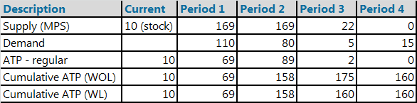
ATP regular (also known as ATP discrete)
-
For the first period, the ATP is the sum of beginning inventory (on hand) plus the supply for the first period (in this case 0) minus the demand for the first period and all the periods following up to, but not including, the next period when supply is planned (in this example period 3).
Note that the ATP for only the first period could be negative. If any of the other periods results in a negative ATP on the first pass, then the system reduces all the prior ATP results until it equals zero OR you get to the first period.
ATP for period 1 = (STOCK + SUPPLY(1) - DEMAND(1) = (10 + 169) - 110 = 69
-
For all periods after the first there are two possibilities:
-
If a demand quantity has been scheduled for the period, the ATP is the supply quantity less all the demand quantities for the period and all demand in subsequent periods until the next supply is scheduled.
-
If no supply quantity is scheduled for a period then the ATP is zero even if there is demand.
ATP for period 3 = SUPPLY(3) - (DEMAND(3) + DEMAND(4)) = 22 - (5 + 15) = 2
The above takes demand in both 3 and 4 as there is no supply in period 4. If the demand is greater than the supply then the ATP is set to 0 and it is rolled back to the previous period. This continues until period 0 and if the result is still negative then the ATP is negative.
-
-
-
Cumulative ATP (WOL)
ATP (WOL) indicates Available to Promise Without Look-Ahead.
The Cumulative ATP without look-ahead equals the ATP in the previous period plus the demand less the supply for that period. The difference between this and normal ATP (discrete) is that in any period it is likely to include units also included in the ATP of other periods.
ATP for period 1 = (STOCK + SUPPLY(1)) - DEMAND(1) = (10 + 169) - 110 = 69
ATP for period 2 = (ATP(2) + SUPPLY(2)) - DEMAND(2) = (69 + 169) - 80 = 158
-
Cumulative ATP (WL)
The difference between this and cumulative ATP WOL is that the quantity produced in one period and committed for use in a future period are omitted from the ATP in all periods preceding that in which they are promised. The ATP (WL) for any period = the ATP (WL) of the preceding period plus the supply of the current period minus the demand of the period minus the sum of the differences between supply and demand for all future periods up to but not including the period from which supply exceeds demand.
SYSPRO does not use this method.
|
|
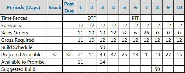
The available to promise for the first period is calculated as the stock on hand less the sales orders up to the next build schedule or the planning time fence (whichever is earlier).
There is a build schedule in period 3, therefore, the calculation is performed as the stock on hand (32) less the sales orders in period 1 (11), less the sales orders in period 2 (10), to give an available to promise figure of 11 in period 1.
The available to promise calculation is restarted at period 3 because a build schedule appears in this period. The available to promise for periods other than the first period is calculated as the build schedule less the sales orders up to the next build schedule, or the planning time fence (whichever is earlier).
Therefore, take the build schedule (50) and subtract the sales orders for period 3 (10), 4 (12), 5 (8) and 6 (6). This gives an available to promise of 14 in period 3.
|
|
|
|
We stopped at period 6 because this is the period that contains the planning time fence. |
|
This displays information for the Stock code selected.
See Bought-out at warehouse level considerations in the Notes and warnings section.
This displays the individual supply and demand that affects the available to promise for the stock item.
| Column | Description |
|---|---|
| Date | Indicates the date of the supply or demand. |
| Reference |
Indicates the source of the supply or demand (e.g. stock, purchase, job, sales order). It includes any Deplete oldest rev/rel material allocations, which indicates that there are more possible demands for the stock code and rev/rel (that will be specified at the time of the kit issue only). |
| Demand qty | Indicates the quantity to be shipped. Job allocations for by-poducts are displayed as negative demand. |
| Supply qty | Indicates the quantity to be received or on hand. |
| Proj on hand |
Indicates the projected on hand balance. This is calculated as the (quantity available + the supply) for each period less the demand for each period. The result is carried forward to the next period. |
| ATP regular | Indicates the quantity available in the current period. For the first period, this equals the stock on hand plus the supply in the current period less the demand in the current period up to the next build schedule or the planning time fence (whichever is earlier). This could be negative in the first period. If any of the other periods results in a negative ATP on the first pass, then the system reduces all the prior ATP results until it equals zero OR you get to the first period. For all subsequent periods it is one of the following:
|
| ATP cumulative |
Indicates the cumulative quantity available without look-ahead. This equals the ATP in the previous period plus the supply in the current period less the demand in the current period. This means it can include units also included in the ATP of other periods. The difference between this and normal ATP (discrete) is that in any period it is likely to include units also included in the ATP of other periods. Refer to Sample calculations for an example. |
-
When this program is accessed from the Requirements Planning Query program, the available to promise details using the Requirements Planning snapshot files/tables is displayed. The word Snapshot is added to the window heading to indicate that the information relates to the snapshot data.
-
If an item is defined as bought-out at warehouse level (Inventory Warehouse Maintenance for Stock Code) then the supplier and lead time defined against the warehouse is used to calculate the various time fences instead of the values held against the stock code.
Generate ATP in MPS mode
This enables you to indicate that the supply of an item must be generated from the build schedule.
-
From the Inventory ATP Query program, select MPS from the Options menu.
Generate ATP in non-MPS mode
This enables you to indicate that the supply of an item must be generated from jobs and purchase orders. You cannot perform this task for non-MPS items because the supply of the item can only be established from jobs and purchase orders (i.e. the build schedule is ignored).
-
From the Inventory ATP Query program, select Non-MPS from the Options menu.